
BinarAlt planner
A browser-based planner with ephemerides, lunar constraints, live observatory weather and an interactive exposure timeline.
Package for ANalysis Of RApidly rotating MAssive stars:
one environment from the observing plan to the 3D model.
Massive stars are frequently very rapid rotators, and most of them live in binary or multiple systems. Rotation flattens them into a Roche shape, makes the surface temperature and gravity depend on latitude through gravity darkening, and broadens and reshapes their spectral lines. Standard one-dimensional, non-rotating analyses are often not enough to interpret what we observe.
Studying these stars also means going through a long analysis chain: planning observing campaigns, handling and normalising the spectra, measuring line profiles and broadening, modelling the distorted star and preparing the results for publication. Each step is usually done with a different tool, written in a different language, with its own formats and conventions, which makes the analysis hard to keep consistent and to reproduce.
PANORAMA (Package for ANalysis Of RApidly rotating MAssive stars) brings the entire analysis workflow into a single Python environment. Developed from scratch as a modular framework, it provides independent tools for each stage of the analysis while maintaining consistent conventions across the package. Explicit input validation, comprehensive documentation, and a ready-to-run demos make the workflow reproducible and easy to adopt, from detailed studies of individual objects to the analysis of large observing campaigns.
The whole analysis chain of a rotating massive star, one module per step.
obs).continuum algorithm, interactively or in batch for large samples (spec).fitline, iacob_broad).rot).specblur).units, tex).| Module | Area | Functions |
|---|---|---|
obs | Observational planning and observing logs | sky_dist, estimate_exposure, estimate_SNR, fits_catalog, periodic_event, obs_phase, obs_phase_night, telescope_pointing, binaralt |
spec | Spectra management | readspec, plotspec, rmvspec, normspec |
fitline | Fitting and characterisation of spectral lines | fitline, fitline_bin |
iacob_broad | v sin i and macroturbulence (FT + GOF) | iacob_broad |
rot | Physics of rotating stars | rpole_to_requator, requator_to_rpole, rpole_to_requiv, requator_to_requiv, rpole_to_rsurf, requator_to_rsurf, vrot_crit, angularrot_crit, rot_rate, rot_rate_angular, rot_params |
broad | Spectral broadening and degradation (in development) | estimate_snr, snrblur, resample, resbroad, rotbroad, macbroad |
units | Physical conversions | wl2kmps, kmps2wl, wl2kmps_rel, kmps2wl_rel, vac2air, air2vac, R2kmps, eddington |
tex | Papers utilities | nobib, queryviz, read_pkl |
What sets PANORAMA apart: from reliable measurements to a consistent physical model.
A browser-based planner with ephemerides, lunar constraints, live observatory weather and an interactive exposure timeline.
Remove artefacts and normalise the continuum IRAF-style, either interactively or in batch for large samples.
Every line fit comes with residual diagnostics, MCMC posteriors and an automatic PASS / WARN / FAIL assessment with advice.
A port of the IDL tool by S. Simón-Díaz: each stage is saved to disk and reused, and save files of the original version can be read.
Classical and MCMC uncertainties are computed and propagated in the analysis of stellar parameters.
A single 3D surface model provides both the line profiles (SPAMMS) and the interferometric models needed to fit the observations.
From planning the night to measuring the lines and modelling the rotating star.
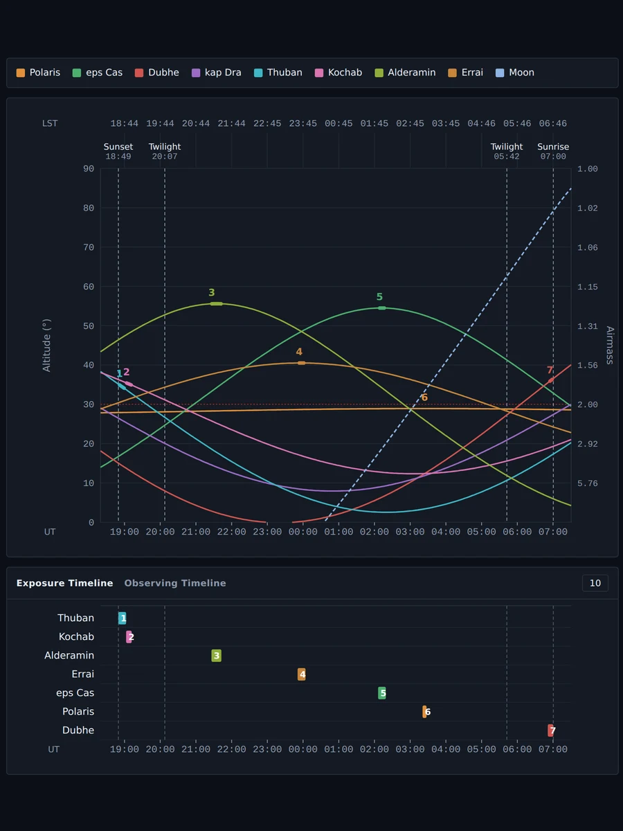
Plot the visibility of your targets for any night and organize the observing sequence around their visibility windows. During the observing session, follow the night in real time with live ephemerides, countdowns, and timing information.
Try the web version with the buttons above; live weather data requires launching the local service from PANORAMA.
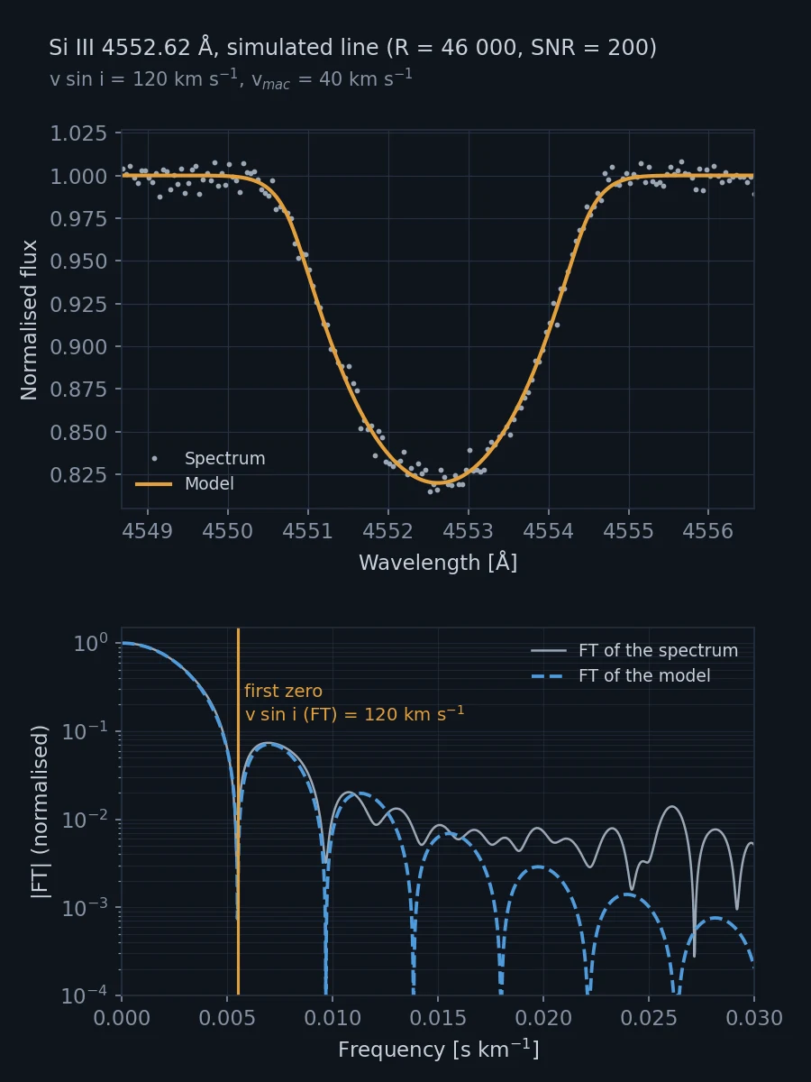
In OB stars, rotation and macroturbulence broaden the lines by similar amounts and are hard to tell apart by eye. Rotation, however, leaves a clear signature: its Fourier transform drops to zero at a frequency set only by v sin i.
A goodness-of-fit over a grid of rotation and macroturbulence profiles then gives both velocities with their uncertainties.
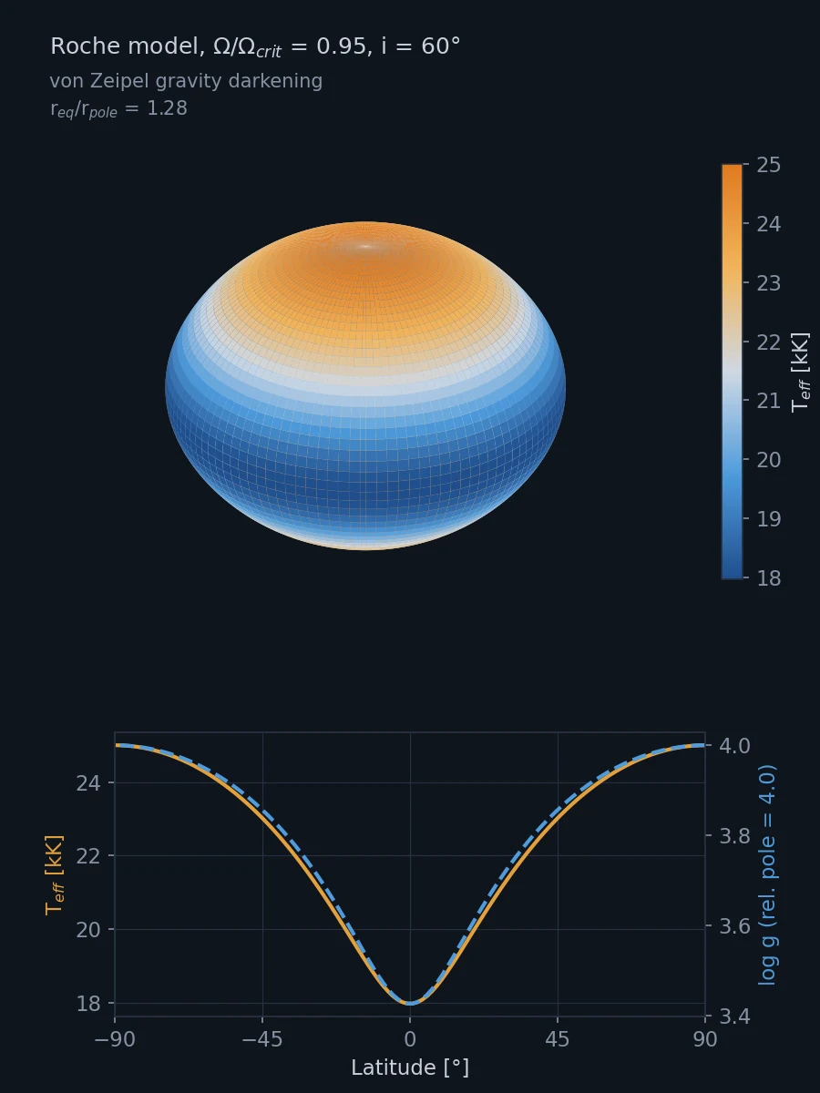
Close to its critical velocity, a star stops being a sphere. The centrifugal force pushes the equator outwards, lowering the effective gravity there, while the poles remain more compact and experience stronger gravity.
Gravity darkening then turns this gravity contrast into a temperature contrast between poles and equator, making the poles hotter while the equatorial regions become cooler.